SysML State Machine Diagrams Explained with an Oscillating Fan Example

State machine diagrams in SysML are one of the best tools for modeling how a system changes behavior over time. They help engineers describe system modes, valid transitions, trigger events, guards, and internal behaviors in a way that is both visual and executable.

In this tutorial, we will walk through the basics of SysML state machine diagrams, then apply those concepts to a practical example: an oscillating fan. Along the way, we will explore how to simulate the state machine, refine it when issues are discovered, and improve the model so it better reflects real-world system behavior.

Watch the full video here:

https://www.youtube.com/watch?v=RRd8qa-T6VQ

---

What Is a State Machine Diagram in SysML?

A SysML state machine diagram is a behavioral diagram used to show how a system moves between different states in response to events, conditions, and actions.

State machine diagrams are useful when a system:

• operates in distinct modes

• responds to external triggers

• has logic that depends on current state

• must remember previous conditions or modes

Examples include:

• fans switching between speed settings

• vehicles changing modes

• controllers responding to input signals

• devices powering on, off, or resuming operation

---

Key Concepts in SysML State Machine Diagrams

Before jumping into the fan example, it helps to understand the core modeling elements.

States and Pseudostates

A state represents a condition or mode the system can be in.

Examples:

• Unpowered

• Off

• Low Speed

• Medium Speed

• High Speed

• Oscillating

• Static

A pseudostate is a special control element used for flow logic, such as:

• initial state

• final state

• shallow history

• deep history

• fork and merge nodes

These help define how execution starts, ends, or resumes.

---

Transitions

A transition is the path from one state to another.

Transitions are usually triggered by:

• signals

• events

• conditions being met

For example, a fan might transition from Off to Low Speed when the user rotates the knob.

---

Guards

A guard is a condition that must be true before a transition can occur.

For example:

x > 5

If the guard condition is false, the transition does not happen.

Guards are useful for modeling decision logic and preventing invalid state changes.

---

Effects

An effect is behavior that occurs during a transition.

For example, when moving from one state to another, the system might update a variable such as:

• RPM

• power draw

• current mode

• timer value

This allows the state machine to influence system properties directly.

---

Shallow History vs Deep History

History pseudostates allow a system to remember where it was before leaving a composite state.

• Shallow history remembers the last top-level substate

• Deep history remembers the nested state within a state

This becomes important when a system powers off and later powers back on.

---

A Simple State Machine Simulation Example

Before looking at the oscillating fan, the video starts with a smaller example to demonstrate transitions, guards, effects, and history behavior.

This example shows how:

• a signal triggers a transition

• a guard evaluates whether a condition is true

• an effect updates a variable

• shallow and deep history produce different results

This is a useful foundation because it shows how state machines are more than just boxes and arrows. They can execute logic and remember prior behavior.

---

Oscillating Fan Example: Modeling a Real System in SysML

The main real-world example in the tutorial is an oscillating fan.

This is a great example for SysML because the fan has multiple interacting modes:

• powered vs unpowered

• off, low, medium, high speed

• oscillating vs static

These modes can exist in parallel, which makes the fan a strong candidate for a state machine with orthogonal regions.

---

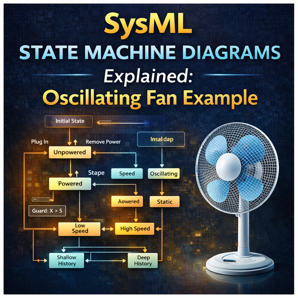
First Pass: Initial State Machine for the Fan

The first version of the state machine captures basic behavior:

• the fan starts unpowered

• plugging it in transitions it to a powered state

• speed signals move it between off, low, medium, and high

• another signal controls oscillating vs static

At first glance, this works reasonably well in simulation.

But when the model is tested more carefully, a problem appears.

If the fan is unplugged while in a specific combination of states, such as:

• High Speed

• Static

and then plugged back in, the model resets to:

• Off

• Oscillating

That is not how the real fan behaves.

This is an important lesson in SysML behavioral modeling: simulation often reveals flaws that are not obvious by looking at the diagram alone.

---

Why the First Fan State Machine Was Incomplete

The first model failed because it did not preserve the last mechanical settings of the fan.

In the real system:

• the knob position remains where the user left it

• the oscillate/static mechanism also remains where it was set

So if the fan is unplugged and plugged back in again, it should return to the previous combination of states.

That means the model needs refinement.

---

Refining the State Machine Diagram

The second version of the fan state machine is more refined and more realistic.

It improves the model by:

• preserving prior settings when power is removed and restored

• associating the state machine with structure

• updating value properties such as RPM and power draw

• adding internal behaviors to states

This is a major step forward because the model now connects behavior to system properties.

---

Running a State Machine With Context

One of the most important differences shown in the tutorial is the difference between running:

• the behavior alone

• the behavior with context

Running without context executes only the state machine logic.

Running with context associates the behavior with a structural block that contains value properties such as:

• powered

• rpm

• power

This allows the simulation to show not just which state the fan is in, but also how those states affect real system values.

For example:

• Low Speed may set RPM to 600

• High Speed may set RPM to 800

• Unpowered may set both RPM and power to zero

This is where the state machine becomes much more useful for system analysis.

---

Entry, Do, and Exit Behaviors in SysML States

A powerful feature of SysML state machine diagrams is the ability to attach behaviors directly to states.

Each state can have:

• Entry behavior — runs when entering the state

• Do behavior — runs while the state remains active

• Exit behavior — runs when leaving the state

The video demonstrates how these behave differently.

Entry Behavior

Runs once when the state is entered.

Exit Behavior

Runs once when leaving the state.

Do Behavior

Runs while the state is active and can be interrupted by incoming triggers.

This distinction matters a lot in simulation.

For example:

• entry and exit behaviors are not interruptible

• do behaviors are interruptible

That makes do behaviors useful for activities that continue while the system remains in a state.

---

Opaque Behaviors vs Activity Diagrams

The fan example uses opaque behaviors to quickly update values like RPM and power.

An opaque behavior is a lightweight way to define logic, often with a simple script or math expression.

For example:

• if powered = true, set RPM to 800

• otherwise set RPM to 0

This works well for simple logic.

But as behavior becomes more complex, it is often better to replace an opaque behavior with an activity diagram.

The tutorial shows how to do exactly that:

• create an activity diagram

• move the logic into the activity

• assign that activity as the entry behavior of a state

This is a useful modeling pattern because it allows the model to grow in complexity without becoming hard to manage.

---

Orthogonal States in SysML

The oscillating fan example also demonstrates orthogonal states, which allow multiple regions of behavior to exist in parallel.

For the fan, that means the system can simultaneously be in:

• one speed state

• one oscillation state

For example:

• High Speed + Static

• Medium Speed + Oscillating

Orthogonal regions are essential when a system has multiple independent but concurrent aspects of behavior.

Without them, the state machine would become much larger and harder to maintain.

---

Finding and Fixing Errors Through Simulation

One of the best parts of this example is that the simulation reveals a real modeling issue.

Even after the refined model is created, another bug is discovered:

when the fan is powered back on in certain speed states, the RPM and power values do not automatically restore correctly.

That leads to further refinement.

Two possible solutions are explored:

• using a do activity to continuously update values

• using a self-transition triggered by the plug-in signal so the entry behavior re-executes

This is exactly how real modeling work happens:

1. create a first pass

2. simulate it

3. discover issues

4. refine the logic

5. simulate again

That iterative loop is at the heart of effective MBSE.

---

Deep History and an Open Modeling Challenge

The tutorial ends with an interesting unresolved challenge involving deep history and orthogonal states.

The goal is to restore both:

• the previous speed state

• the previous oscillation/static state

Deep history seems promising, but in this case it only restores one orthogonal region correctly, not both.

Several approaches are attempted, including:

• multiple history nodes

• fork pseudostates

• multiple transitions with the same signal

But none fully solve the problem in the demonstrated model.

That makes this a valuable example not just of how state machines work, but also of where tool behavior and modeling execution semantics can become tricky.

---

Best Practices for SysML State Machine Diagrams

Based on this example, here are a few practical best practices.

Start simple

Build a first-pass state machine before trying to capture every detail.

Simulate early

State machine simulations often reveal logic problems quickly.

Associate behavior with structure

Use context when you need state changes to affect system value properties.

Use orthogonal regions carefully

They are powerful, but they can complicate history and restoration logic.

Move beyond opaque behaviors when needed

Use activity diagrams when state logic becomes more sophisticated.

Refine iteratively

Good state machines are usually built through several rounds of improvement.

---

Final Thoughts

SysML state machine diagrams are one of the most powerful behavioral modeling tools available in MBSE. They help engineers define system modes, valid transitions, internal actions, and dynamic behavior in a way that can be simulated and improved over time.

The oscillating fan example shows why that matters. A simple first-pass model may seem correct at first, but simulation helps uncover flaws, refine logic, and better align the model with how the real system behaves.

If you want to get better at SysML state machine modeling, this is exactly the kind of hands-on example worth practicing.

Watch the full walkthrough here:

https://www.youtube.com/watch?v=RRd8qa-T6VQ